When doing statistical hypothesis testing, the math behind it gives us the toolset to determine the statistical significance of our observations. But if we're doing a two-sample test on a simple hypothesis, eg.  $H_{0}:\mu_{1}=\mu_{2}$ vs. $H_{1}:\mu_{1}\ne\mu_{2}$ rejecting it won't tell us anything about the magnitude of the difference.

Usually, aside from making sure that the difference in measurements you observed are statistically significant, you want your observed differences to be practically significant as well. That means you don't want to test simply if your statistics (e.g. averages) differ, but you want them to differ by some margin, $\epsilon$. The size of the margin is dependent on the application - if you want to increase a click-through rate you probably have a business goal clearly specified, saying something like Increase CTR by 10 percentage points.

So how do we do test for a margin of difference? We'll need to run what's called a composite hypothesis test.

It's a fun practice in fundamentals of hypothesis testing to derive the formulas behind it, so let's first derive the test for the case of a single sample, comparing its mean to a constant. Then we'll modify it to make a two-sample test, enabling us to compare averages of two samples.

One-sample test

Let's assume our data points $X_{1},X_{2},...,X_{n}$ come as iid observations from some unknown distribution, with mean $\mu$ and variance $\sigma^2$. We want to test with the following null and alternative hypotheses

\[ \begin{eqnarray*} H_{0}:\left|\mu-\mu_{0}\right| & \le & \epsilon\\ H_{1}:\left|\mu-\mu_{0}\right| & > & \epsilon \end{eqnarray*} \]

where $\epsilon > 0$ is a constant quantifying our desired practical significance.

Unrolling this, we get

$H_{0}:(\mu\ge\mu_{0}-\epsilon)\ and\ (\mu\le\mu_{0}+\epsilon)$
$H_{1}:(\mu<\mu_{0}-\epsilon)\ and\ (\mu>\mu_{0}+\epsilon)$

which should make it obvious why it's called a composite hypothesis test.

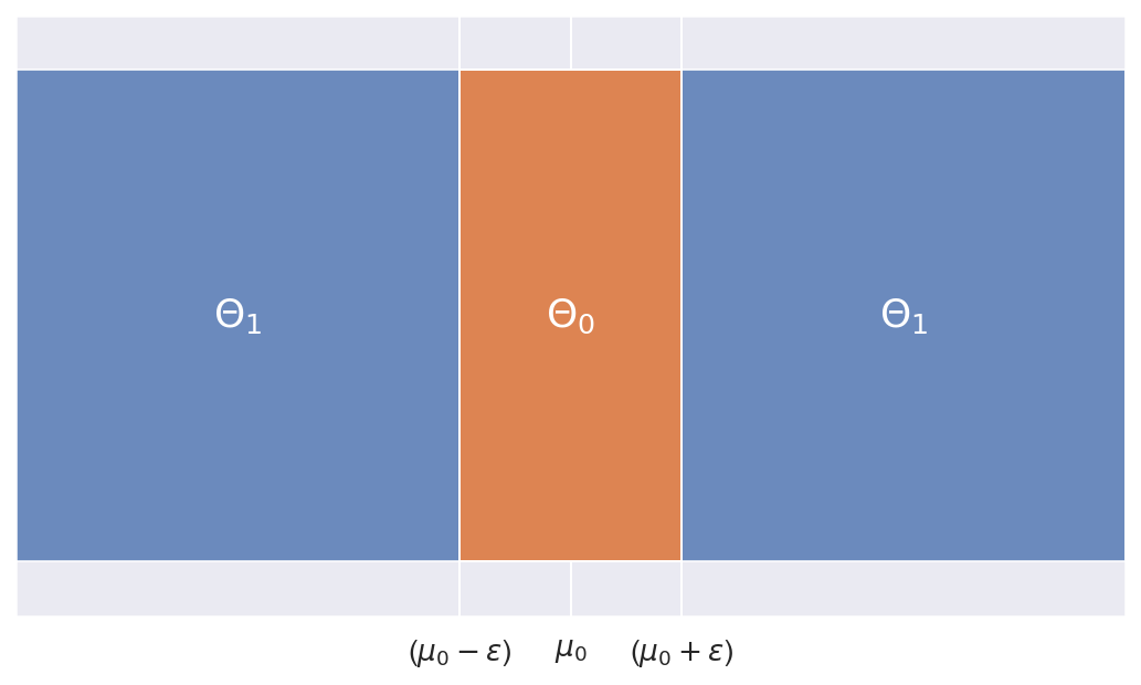
As usual, we'll partition the parameter space $\Theta$ into two subspaces, corresponding to parameter spaces for $H_0$ and $H_1$:

$\Theta_{0}=\left\{ \mu\in\mathbb{\mathbb{R}}\mid(\mu\ge\mu_{0}-\epsilon)\ and\ (\mu\le\mu_{0}+\epsilon)\right\} $
$\Theta_{1}=\left\{ \mu\in\mathbb{\mathbb{R}}\mid(\mu<\mu_{0}-\epsilon)\ and\ (\mu>\mu_{0}+\epsilon)\right\} $

Since we want to test the mean, we'll use sample average as the estimate for  $\mu$:

\[
\hat{\mu}=\bar{X}_{n}=\frac{1}{n}\sum_{i=1}^{n}X_{i}
\]

Central limit theorem tells us that as $n$ grows, $\bar{X}_n$ converges in distribution to a normal random variable:

\[
n\rightarrow\infty:\ \sqrt{n}(\bar{X}_{n}-\mu)\overset{i.d}{\rightarrow}\mathcal{N}\left(0,\sigma^{2}\right)
\]

and the Continuous mapping theorem allows us to go back and forth and get that:

\[n\rightarrow\infty:\ \bar{X}_{n}\overset{i.d}{\rightarrow}\mathcal{N}\left(\mu,\frac{\sigma^{2}}{n}\right)\]

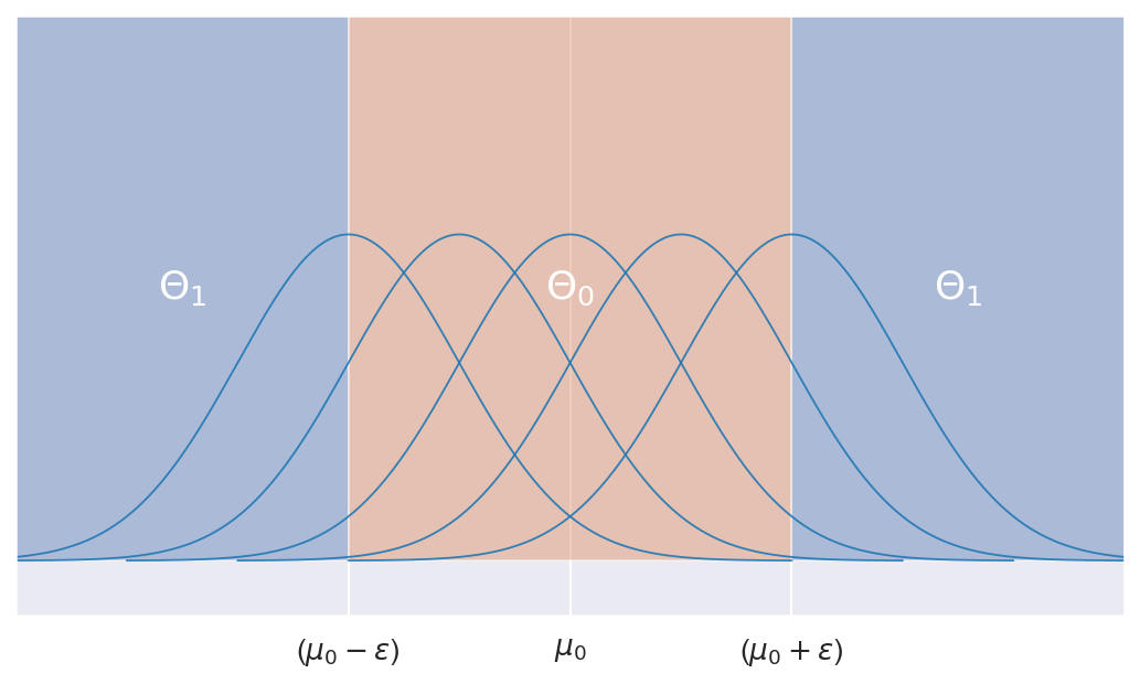
So under $H_0$, $\bar{X}_n$ can be asymptotically distributed as any of the $\mathcal{N}\left(\mu,\frac{\sigma^{2}}{n}\right)$ for $\mu\in\Theta_{0}$

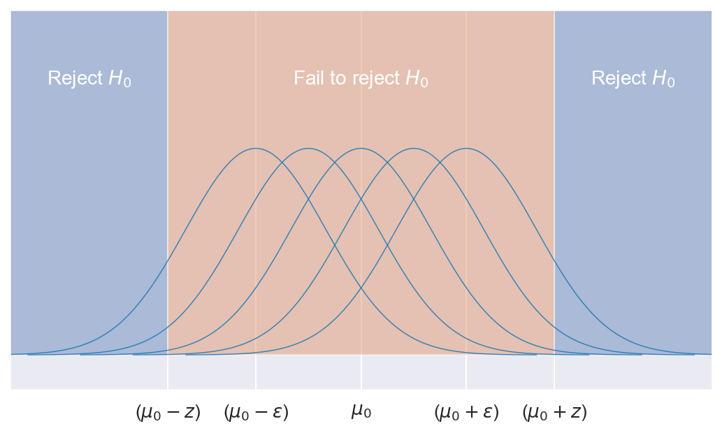
We want to design a test with significance level $\alpha$, limiting the Type 1 error. Let's consider the following test for some $z \ge \epsilon$:

\[\psi=\begin{cases}1\ (H_{0}\ rejected) & if\ (\hat{\mu}\le\mu_{0}-z)\ or\ (\hat{\mu}\ge\mu_{0}+z)\\0\ (H_{0}\ not\ rejected) & otherwise \end{cases}\]

We denote as Type I error  the error of falsely rejecting the null hypothesis. Formally, we define the Type I error rate $\alpha_\psi$ as the probability of rejecting the null hypothesis when it was in fact true.

$\alpha_\psi=P_\mu(\psi=1); \mu\in\Theta_0$

The level $\alpha$ of a test is the largest Type I error that we'll get for any $\mu\in\Theta_0$. Formally, a statistical test has level $alpha$ if:

$\alpha_\psi=P_\mu(\psi=1)\le\alpha, \forall\mu\in\Theta_0$

Thus, for our test $\psi$, we have the level

\[ \begin{eqnarray*} \alpha & = & \underset{\mu\in\Theta_{0}}{sup}P_{\mu}\left(\psi=1\right)\\ & = & \underset{\mu\in\Theta_{0}}{sup}P_{\mu}\left((\hat{\mu}<\mu_{0}-z)\ or\ (\hat{\mu}>\mu_{0}+z)\right)\\ & = & \underset{\mu\in\Theta_{0}}{sup}P_{\mu}\left((\hat{\mu}-\mu_{0}<-z)\ or\ (\hat{\mu}-\mu_{0}>z)\right)\\ & \overset{by\ CLT}{\sim} & \underset{\mu\in\Theta_{0}}{sup}\left\{ P\left(\mathcal{N}\left(\mu-\mu_{0},\frac{\sigma^{2}}{n}\right)<-z\right)\ +\ P\left(\mathcal{N}\left(\mu-\mu_{0},\frac{\sigma^{2}}{n}\right)>z\right)\right\} \\ & = & \underset{\mu\in\Theta_{0}}{sup}\left\{ P\left(\mathcal{N}\left(0,1\right)<\sqrt{n}\frac{-z-(\mu-\mu_{0})}{\sigma}\right)\ +\ P\left(\mathcal{N}\left(0,1\right)>\sqrt{n}\frac{z-(\mu-\mu_{0})}{\sigma}\right)\right\} \\ & = & \underset{\mu\in\Theta_{0}}{sup}\left\{ \Phi\left(\sqrt{n}\frac{-z-(\mu-\mu_{0})}{\sigma}\right)+1-\Phi\left(\sqrt{n}\frac{z-(\mu-\mu_{0})}{\sigma}\right)\right\} \\ \end{eqnarray*} \]

Where $\Phi$ is the cumulative distribution function of a standard Gaussian.

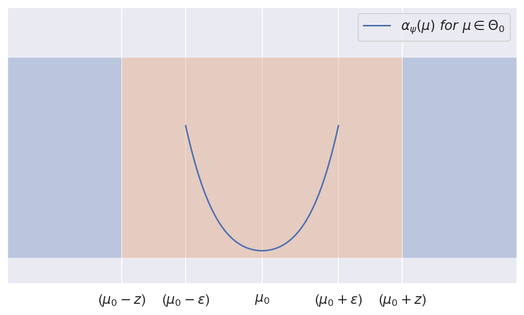
Let's see how $\alpha_\psi$ behaves as we move $\mu$ over $\Theta_0$, that is from $\mu_0-\epsilon$ to $\mu_0+\epsilon$. We'll take the derivative of $\alpha_\psi$ with respect to $\mu$:

\[ \begin{eqnarray*} \frac{\partial}{\partial\mu}\alpha_{\psi}(\mu) & = & \frac{\partial}{\partial\mu}\left(P_{\mu}\left(\psi=1\right)\right)\\ & = & -\phi\left(\sqrt{n}\frac{-z-(\mu-\mu_{0})}{\sigma}\right)\cdot\frac{\sqrt{n}}{\sigma}+\phi\left(\sqrt{n}\frac{z-(\mu-\mu_{0})}{\sigma}\right)\cdot\frac{\sqrt{n}}{\sigma}\\ & = & \frac{\sqrt{n}}{\sigma}\left(\phi\left(\sqrt{n}\frac{z-(\mu-\mu_{0})}{\sigma}\right)-\phi\left(\sqrt{n}\frac{-z-(\mu-\mu_{0})}{\sigma}\right)\right) \end{eqnarray*} \]

Where $\phi(x)=\frac{\partial}{\partial{x}}\Phi(x)$ is the pdf of a standard Gaussian.

We can show by symmetry of $\phi$ that $\frac{\partial}{\partial\mu}\alpha_{\psi}(\mu)=0$ when $\mu=\mu_0$, and using properties of the Gaussian pdf prove that regardless of $n$ and $\sigma$:

$\frac{\partial}{\partial\mu}\alpha_{\psi}(\mu)<0\ for\ \mu<\mu_0$
$\frac{\partial}{\partial\mu}\alpha_{\psi}(\mu)>0\ for\ \mu>\mu_0$

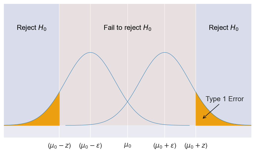
Concretely, this means that our $\alpha_\psi$ is the smallest at $\mu=\mu_0$ and grows as we move away from $\mu_0$. It's easily shown that $\alpha_\psi(\mu_0-\epsilon)=\alpha_\psi(\mu_0+\epsilon)$, ie. it has the same (largest) value at the edges of $\Theta_0$, i.e. when $\mu=\mu_0\pm\epsilon$, or formally:

\[ \begin{eqnarray*} \underset{\mu\in\Theta_{0}}{argsup}P_{\mu}\left(\psi=1\right) & = & \mu_{0}\pm\epsilon\\ \underset{\mu\in\Theta_{0}}{sup}P_{\mu}\left(\psi=1\right) & = & \Phi\left(\sqrt{n}\frac{-z-\epsilon}{\sigma}\right)+1-\Phi\left(\sqrt{n}\frac{z-\epsilon}{\sigma}\right) \end{eqnarray*} \\ \\ \]

So far, we've shown that with our test defined as:

\[\psi=\begin{cases}1\ (H_{0}\ rejected) & if\ (\hat{\mu}<\mu_{0}-z)\ or\ (\hat{\mu}>\mu_{0}+z)\\0\ (H_{0}\ not\ rejected) & otherwise \end{cases}\]

and for an arbitrary $z\ge\epsilon$, our test has level $\alpha=\Phi\left(\sqrt{n}\frac{-z-\epsilon}{\sigma}\right)+1-\Phi\left(\sqrt{n}\frac{z-\epsilon}{\sigma}\right)$.

Let's now go the other way and pick $z$ for a desired level $\alpha$. Looking at the equation for $\alpha$ above, it doesn't look obvious how to find $z$. To avoid solving this equation, we'll note the following: as we move $z$ farther from $\epsilon$ our $\alpha$ gets smaller. That means we can find $z_\alpha$ numerically by bisection method.

However, since getting the p-value is enough for a test, we don't actually need to solve for $z_\alpha$. Note that as $z$ increases, $\alpha$ decreases, and from the definition of our test we have that the largest $z$ at which we'll ever reject is $z=\left|\hat{\mu}-\mu_{0}\right|$. This means that the smallest level at which we can reject is given by:

\[ \text{p-value}=\underset{z\in[\epsilon,\infty]}{min}\alpha=\Phi\left(\sqrt{n}\frac{-\left|\hat{\mu}-\mu_{0}\right|-\epsilon}{\sigma}\right)+1-\Phi\left(\sqrt{n}\frac{\left|\hat{\mu}-\mu_{0}\right|-\epsilon}{\sigma}\right) \]

As a special case, consider the test with $\epsilon=0$. We'll have:

\[ \begin{eqnarray*} H_{0}:\left|\mu-\mu_{0}\right| & = & 0\Leftrightarrow\mu=\mu_{0}\\ H_{1}:\left|\mu-\mu_{0}\right| & > & 0\Leftrightarrow\mu\ne\mu_{0} \end{eqnarray*} \]

and:

\[ \begin{eqnarray*} \text{p-value} & = & \underset{z\in[\epsilon,\infty]}{min}\alpha=\Phi\left(\sqrt{n}\frac{-\left|\hat{\mu}-\mu_{0}\right|}{\sigma}\right)+1-\Phi\left(\sqrt{n}\frac{\left|\hat{\mu}-\mu_{0}\right|}{\sigma}\right)\\ & = & 2\cdot\Phi\left(\sqrt{n}\frac{-\left|\hat{\mu}-\mu_{0}\right|}{\sigma}\right) \end{eqnarray*} \]

which is exactly the simple hypothesis two-sided test.

Two-sample test

So far we've just derived a one-sample test, so we need to modify it a bit to test the difference between means of two samples.

Given $n$ observations $X_1...X_n$ from a distribution with mean $\mu_X$ and variance $\sigma_X^2$, and $m$ observations $Y_1...Y_m$ from a distribution with mean $\mu_Y$ and variance $\sigma_Y^2$ , we formulate the following null and alternative hypotheses:

\[ \begin{eqnarray*} H_{0} & : & \left|\mu_{1}-\mu_{2}\right|\le\epsilon\\ H_{1} & : & \left|\mu_{1}-\mu_{2}\right|>\epsilon \end{eqnarray*} \]

Which is basically saying $\mu_1$ is different from $\mu_2$ by at least a margin of $\epsilon$. We use $\epsilon$ here to state our desired practical significance.

Let's define $d$ as $d=\mu_1-\mu_2$. Then we can rewrite our hypotheses as:

\[ \begin{eqnarray*} H_{0} & : & \left|d-0\right|\le\epsilon\\ H_{1} & : & \left|d-0\right|>\epsilon \end{eqnarray*} \]

We'll use $\hat{d}=\hat{\mu}_{1}-\hat{\mu}_{2}=\bar{X}_{n}-\bar{Y}_{n}$ as the estimator for $d$. From the Central limit theorem and the multivariate delta method, we get that:

\[ \hat{d}=\bar{X}_{n}-\bar{Y}_{n}\overset{i.d.}{\rightarrow}\mathcal{N}\left(\mu_{X}-\mu_{Y},\frac{\sigma_{X}^{2}}{n}+\frac{\sigma_{Y}^{2}}{m}\right) \]

Substituting $\hat{\mu}\rightarrow\hat{d}$, $\mu_0\rightarrow0$, $\frac{\sigma^{2}}{n}\rightarrow\frac{\sigma_{X}^{2}}{n}+\frac{\sigma_{Y}^{2}}{m}$ and plugging into our formula for p-value, we get:

\[ \text{p-value}=\Phi\left(\frac{-\left|\hat{d}\right|-\epsilon}{\sqrt{\frac{\sigma_{X}^{2}}{n}+\frac{\sigma_{Y}^{2}}{m}}}\right)+1-\Phi\left(\frac{\left|\hat{d}\right|-\epsilon}{\sqrt{\frac{\sigma_{X}^{2}}{n}+\frac{\sigma_{Y}^{2}}{m}}}\right) \]

Note once again that setting $\epsilon=0$ we get the familiar form for a simple two-sample two-sided test for difference of means.

Conclusion

We've shown a step-by-step exercise of deriving a two-sample two-sided Z-test with a margin of tolerance. It should be even simpler to derive a one-sided test, as it's just a modification of a simple hypothesis one-sided test with an extended range for $\Theta_0$.

Using the formulas above, in case we're rejecting $H_0$ we can also find the largest $\epsilon$ at which we can reject with a given p-value. This gives us an upper bound on the difference between means for a given statistical significance.